Rare Events

The difference between practice and theory is greater in practice than in theory.

Imagine a square field divided into 25 equal square patches. 100 raindrops come down. For each small square, we expect 4 raindrops on average. This simulation shows that there’s a good number of outcomes one might consider surprising. Some patches get nothing, and some get more than twice the expected amount of water.

A very oversimplified explanation of how extreme drought and extreme flooding can happen right next to one another, in time and space.

Show the code

import pandas as pd
pd.DataFrame(
    index=list('AB'),
    data = {
        'events': [4, 8],
        'non-events': [396, 392],
        'event rate': ['1%', '2%']
    }
)

	events	non-events	event rate
A	4	396	1%
B	8	392	2%

Show the code

import altair as alt
import numpy as np
import pandas as pd

# set random seed for reproducibility
np.random.seed(42)

# event rate
P = 0.01

# 400 experiments, repeated 2500 times
N, R = 400, 2500

df = pd.DataFrame({
    'binomial': np.random.binomial(N, P, R),
    'poisson': np.random.poisson(N*P, R),
})

def pdf_plot(distribution):
    return alt.Chart(
        df, title=distribution,
    ).transform_joinaggregate(
        total='count(*)'
    ).transform_calculate(
        pct='1 / datum.total'
    ).mark_bar().encode(
        alt.X(f'{distribution}:O', title="event count"),
        alt.Y('sum(pct):Q', axis=alt.Axis(format='%'), title="frequency")
    )

pdf_plots = pdf_plot('binomial') | pdf_plot('poisson')
pdf_plots.resolve_scale(y='shared')

Show the code

import numpy as np
import pandas as pd

t10k = pd.DataFrame({
    'x': np.random.randint(0, 100, 100),
    'y': np.random.randint(0, 100, 100),
})
ax = t10k.plot.scatter(
    x='x', y='y', alpha=0.4,
    xlim=(0,100), ylim=(0, 100),
    grid=True, figsize=(4,4),
    title="400 assays with 1% event rate:\nobserved event counts in 25 simulations"
)

for a in range(5):
    for b in range(5):
        n_events = sum((t10k.x // 20 == a) & (t10k.y // 20 == b))
        ax.text(a*20+10, b*20+10, n_events)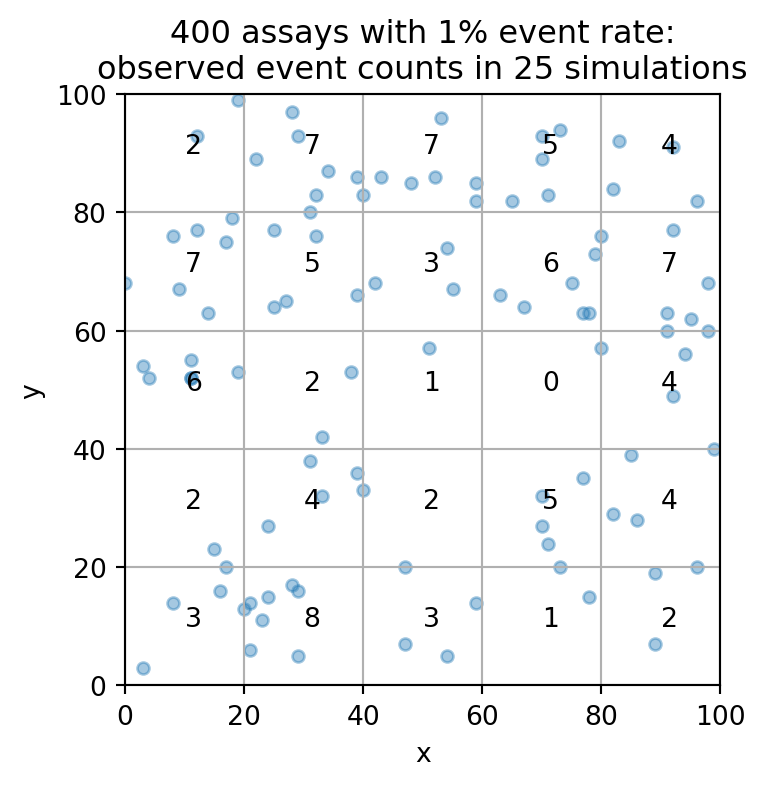

Simulation (HTML5 Canvas)

https://gist.github.com/liquidcarbon/e4db5ab305c57a542136499871f7773d

https://www.linkedin.com/posts/alekis_html5-poisson-statistics-activity-7087531310398767104-zdw3